Data Mining process
Input: numerical visualization
Output: categorical visualization
Output: prediction model analysis
Data Mining process
Input: numerical visualization
Output: categorical visualization
Output: prediction model analysis
The Case Study is based on a hypothetical bank credit risk data set.
The data set contains 26 variables collected on 10,000 observations:
The goal of the Case Study is to analyze the data and to predict the Target Variable “Esito Negativo”.
Click here to see the list of the variables of this Case Study, their possible codes
and their English Translation.
This Case Study is developed with Python Jupyter Notebook to load data and apply models,
and Plotly Dash to build a dashboard to show the results.
Python is a high-level, general-purpose programming language. Its design philosophy emphasizes code readability in particular with the use of significant indentation to define the end of the statements and the blocks of statements.
Python is dynamically-typed and garbage-collected. It supports multiple programming paradigms, including structured (particularly procedural), object-oriented and functional programming.
It is open source and full of comprehensive standard library and user defined modules.
The Jupyter Notebook App is a server-client application that allows editing and running notebook documents via a web browser. The Jupyter Notebook App can be executed on a local desktop requiring no internet access (as described in this document) or can be installed on a remote server and accessed through the internet.
The notebook document allows to associate Python Code and its results in a graphical user-friendly interface.
It's particularly useful to present results of programs interactively modified by the user.
Plotly Dash is a python framework created by Plotly company for creating interactive web applications.
With Dash, you don't have to learn HTML, CSS and Javascript in order to create interactive dashboards, you only need python code.
It's one ot the most used tool to build dashboard with python code.
The present case study is develped in two phases:
Among the models tested to predict the default indicators there are the following:
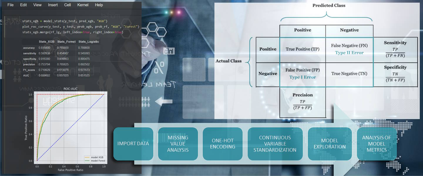
A standard Data Mining process has been developed to load and control the input data, transforming it into actionable dataframes, and to estimate and perform a first comparison.
A Jupyter notebook has been created to:
The Accuracy is the main error indicator used to evaluate the models,
and then Sensitivity, Specificity, F1-Score, AUC and precision indicators.
ROC charts have been plotted to manually compare the results.
The picture below describes the standard data mining process steps followed to build data, models and evaluate results.


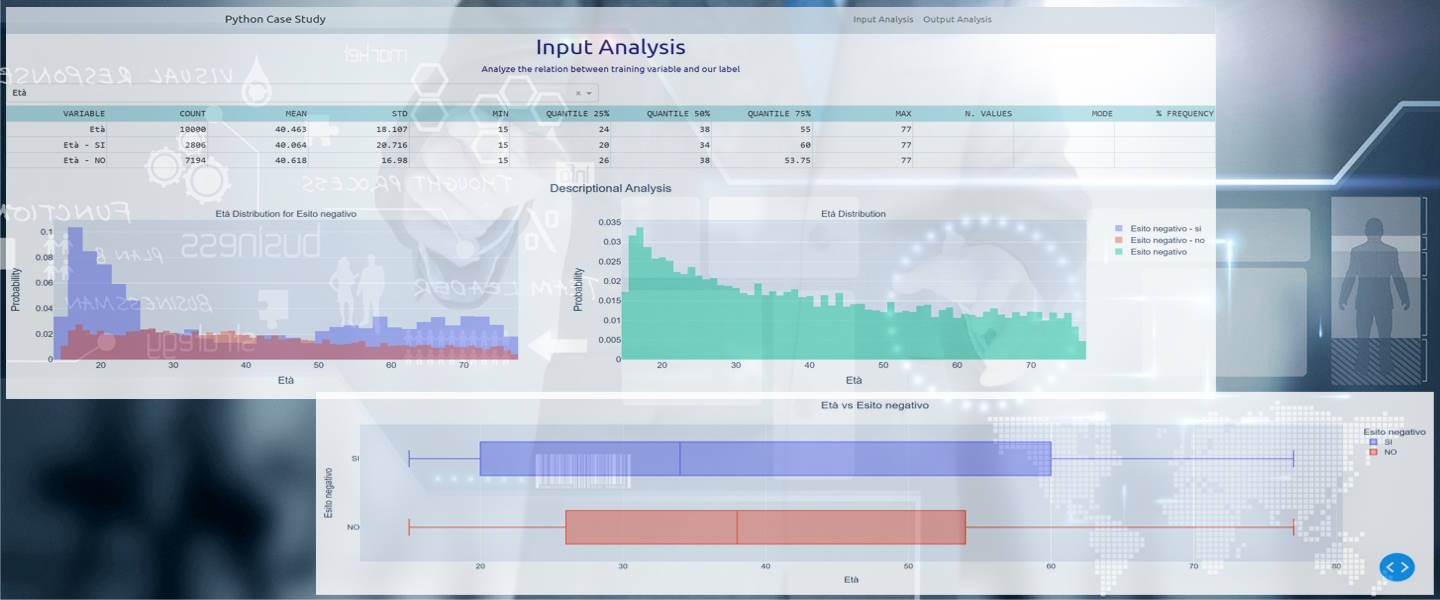
A interactive dashboard illustrates some statistical indicators and probability distribution in a easy way.
The user can select one of the available variables in the input sample.
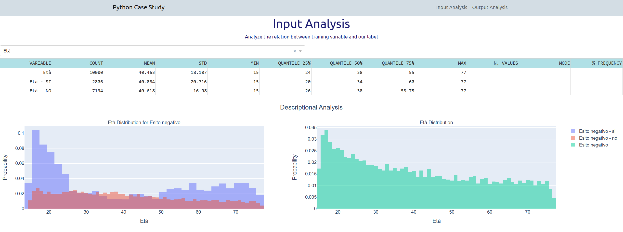
If the variable is numerical and continuos, as the selected variable below Età, the user can see:
The latter with all the values in green colour.
The two histograms provide a vision of how the cases are distributed
respect the categorical values of the selected variable.
In the example below the histograms prove that the most risky categories are the young and older people.
The BoxPlot chart provides a different perspective, with a synthesis of most of the basic statistics
illustrated in the table above the charts, giving an idea of the importance of the two tails
and of the concentration of the values around the median.
In particular in this example, with the variable Età, we obtain a different vision of the distribution
that hides the concentration of the most risky cases in the young and older people.
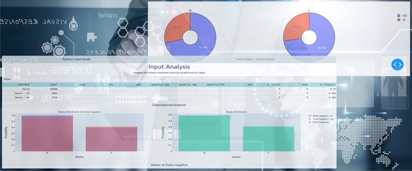
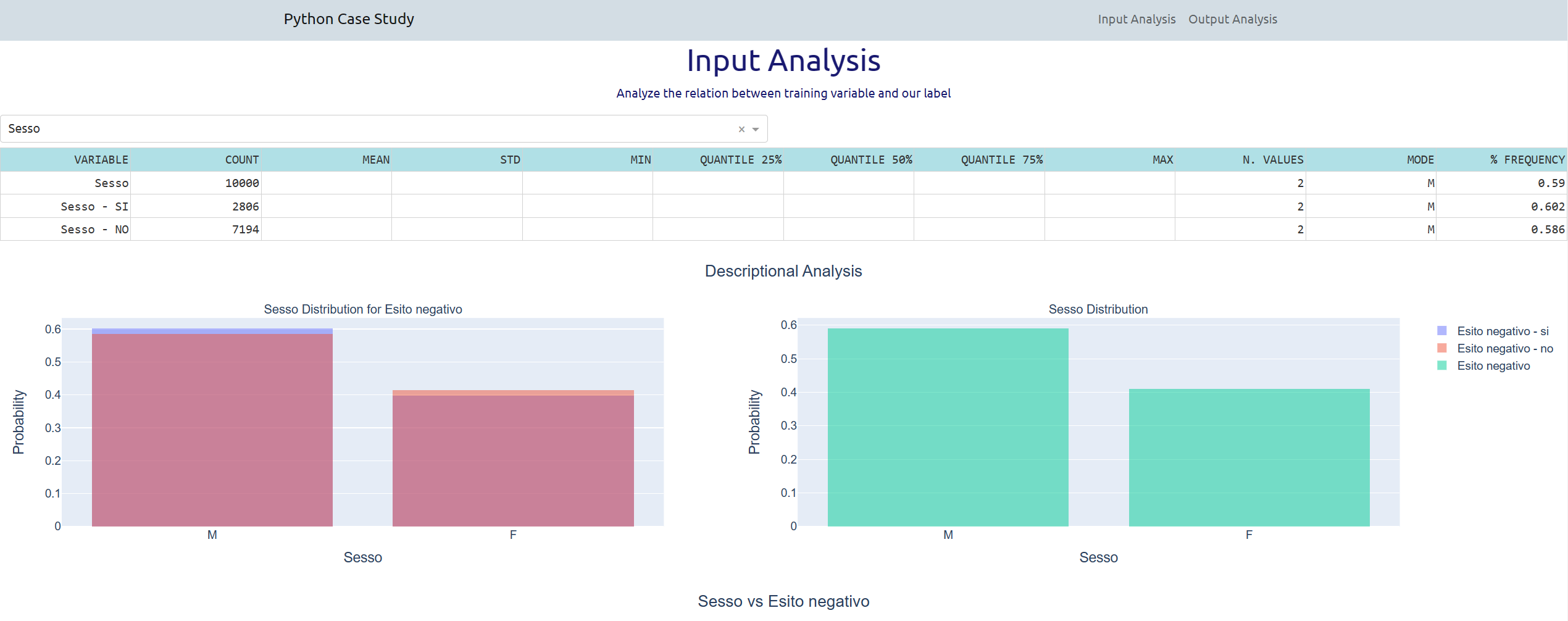
If the variable is categorical, as the selected variable below Sesso, the user can see:
The latter with all the values in green colour.
The two histograms provide a vision of how the cases are distributed
respect the categorical values of the selected variable.
In the example below the histograms prove that the most risky categories
are the male people for a small amount.
In particular in this example, the Male people have higher percentage for a slight amount of about 1%.
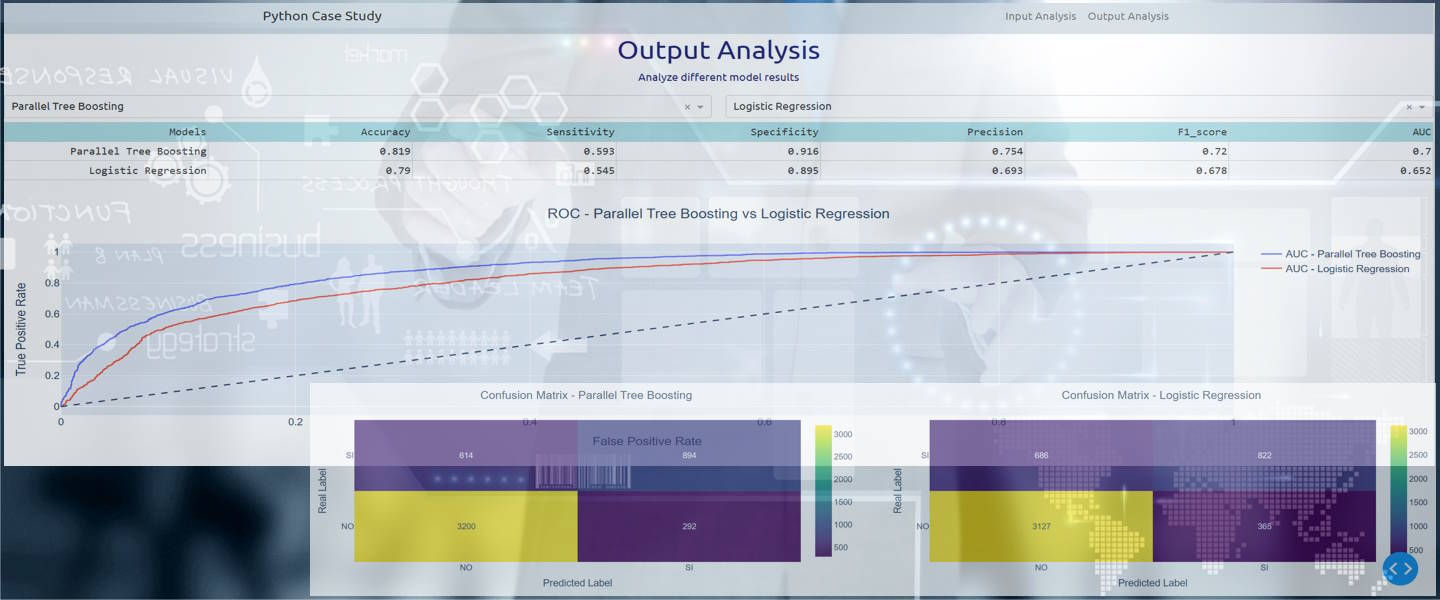
The section about output analysis of the interactive dashboard
compares the results of the 4 statistical models.
The user has to select two models to be compared.
Like in the example below where the models Parallel Tree Boosting and Logistic Regression
are selected.
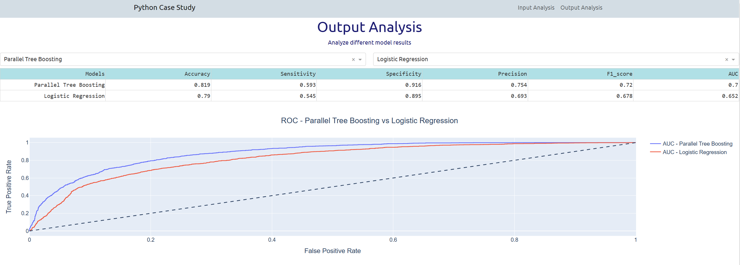
The table in the right summerizes the main basic indicators and numbers used to evaluate models.
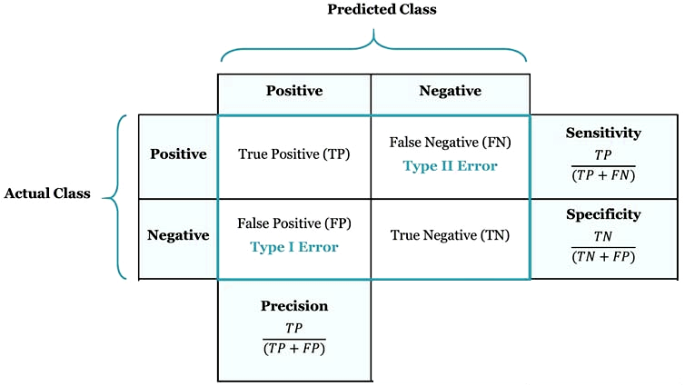
Where:
Then in the DashBoard outputs are shown:
The computed error or performance indicators are:
-Accuracy: the number of correct predition on the total.
Otherwise the number of TruePositive+TrueNegative on the total.
-Sensitivity: (or True Positive Rate or Recall) the proportion of positive data points
that are correctly considered as positive, with respect to all positive data points.
Otherwise the number of TruePositive on the sum of FalseNegative and TruePositive.
-Specificity: (or False Positive Rate) the proportion of negative data points
that are correctly considered as negative, with respect to all negative data points.
Otherwise the number of TrueNegative on the sum of FalsePositive and TrueNegative.
-Precision: It is the number of correct positive results divided by the number
of positive results predicted by the model.
Otherwise the number of TruePositive on the sum of FalsePositive and TruePositive.
-F1_score: F1 Score is the Harmonic Mean between precision and recall.
The range for F1 Score is [0, 1]. It tells you how precise your classifier is
(how many instances it classifies correctly), as well as how robust it is
(it does not miss a significant number of instances).
Otherwise is 2 divided by then sum of 1/Precision and 1/Recall.
-AUC: (or Area Under Curve) AUC is the area under the curve of plot False Positive Rate
vs True Positive Rate at different points in [0, 1]. AUC has a range of [0, 1].
AUC is one of the most widely used metrics for evaluation, used for binary classification problem.
AUC of a classifier is equal to the probability that the classifier will rank
a randomly chosen positive case higher than a negative one.
For all these indicators, the greater the value, the better is the performance of our model.
The confusion matrix allows you to evaluate graphically a model in term of number
or percentage of cases falling in the four sector,
where tipically the most important sector is the one in the upper right
with the true positive events detected by the model, the default of the client in this case.
The second sector in importance if the true negative events.

Between the two selected models in the example above,
the Parallel Tree Boosting is always better than the Logistic Regression,
easily to imagine considering that the Boosting has more parameters to fit the model
and requires more time to detect the best Tree sub model.
Click on the video below to see the dashboard in action
for the visualization of the values of each column of a selected data set
and to see a quick view of the component data flow that generates and controls the dashboard.